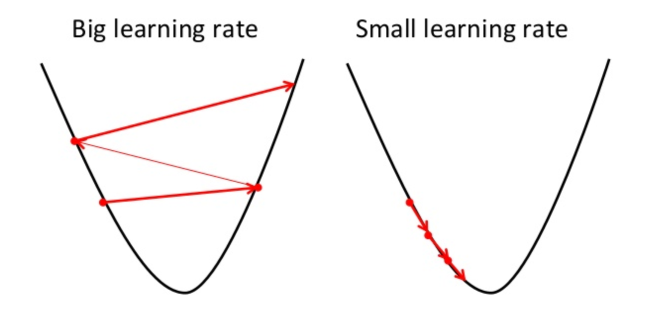
But becoming familiar with the structure of a GLM is essential for parameter tuning and model selection. Eventually, with enough small steps in the direction of the gradient, which is the steepest descent, it will end up at the bottom of the hill. It models $P(\mathbf{x}_i|y)$ and makes explicit assumptions on its distribution (e.g. What is the name of this threaded tube with screws at each end? While this modeling approach is easily interpreted, efficiently implemented, and capable of accurately capturing many linear relationships, it does come with several significant limitations. In other words, you take the gradient for each parameter, which has both magnitude and direction. The best parameters are estimated using gradient ascent (e.g., maximizing log-likelihood) or descent (e.g., minimizing cross-entropy loss), where the chosen objective (e.g., cost, loss, etc.) p &= \sigma(f) \cr When you see i and j with lowercase italic x (xi,j) in Figures 8 and 10, the value is a representation of a jth feature in an ith (a single feature vector) instance. The key takeaway is that log-odds are unbounded (-infinity to +infinity). \end{eqnarray}. Because the log-likelihood function is concave, eventually, the small uphill steps will reach the global maximum. $$\eqalign{ And using the gradient descent algorithm, we update the parameters until they converge to their optima. Asking for help, clarification, or responding to other answers. differentiable or subdifferentiable).It can be regarded as a stochastic approximation of gradient descent optimization, since it replaces the actual gradient (calculated from the entire data set) by Asking for help, clarification, or responding to other answers. (10 points) 2. Why is this important? )$. How to assess cold water boating/canoeing safety. When did Albertus Magnus write 'On Animals'? If we summarize all the above steps, we can use the formula:-. 3 0 obj << I cannot for the life of me figure out how the partial derivatives for each weight look like (I need to implement them in Python). WebPoisson distribution is a distribution over non-negative integers with a single parameter 0. We take the partial derivative of the log-likelihood function with respect to each parameter. However, the third equation you have written: l ( ) j = ( y 1 h ( x 1)) x j 1. is not the gradient with respect to the loss, but the gradient with respect to the log likelihood! exact l.s. \]. Think of it as a helper algorithm, enabling us to find the best formulation of our ML model. Logistic regression has two phases: training: We train the system (specically the weights w and b) using stochastic gradient descent and the cross-entropy loss. d/db(y_i \cdot \log p(x_i)) &=& \log p(x_i) \cdot 0 + y_i \cdot(d/db(\log p(x_i))\\ Of course, I ignored the chain rule for that one! What does Snares mean in Hip-Hop, how is it different from Bars. And because the response is binary (e.g., True vs. False, Yes vs. No, Survived vs. Not Survived), the response variable will have a Bernoulli distribution. The biggest challenge I am facing here is to implement the terms lambda, DK, theta(dk) and theta(dyn) from the equation in the paper. A tip is to use the fact, that $\frac{\partial}{\partial z} \sigma(z) = \sigma(z) (1 - \sigma(z))$. Possible ESD damage on UART pins between nRF52840 and ATmega1284P. Luke 23:44-48. Considering the following functions I'm having a tough time finding the appropriate gradient function for the log-likelihood as defined below: $P(y_k|x) = {\exp\{a_k(x)\}}\big/{\sum_{k'=1}^K \exp\{a_{k'}(x)\}}$, $L(w)=\sum_{n=1}^N\sum_{k=1}^Ky_{nk}\cdot \ln(P(y_k|x_n))$. The next step is to transform odds into log-odds. In the case of linear regression, its simple. Iterating through the training set once was enough to reach the optimal parameters. So it tries to push coefficients to 0, that was the effect has on the gradient, exactly what you expect. To learn more, see our tips on writing great answers. $p(x)$ is a short-hand for $p(y = 1\ |\ x)$. Where you saw how feature scaling, that is scaling all the features to take on similar ranges of values, say between negative 1 and plus 1, how they can help gradient descent to converge faster. So basically I used the product and chain rule to compute the derivative. \begin{align} import numpy as np import pandas as pd import sklearn import In the context of a cost or loss function, the goal is converging to the global minimum. Step 2, we specify the link function. To learn more, see our tips on writing great answers. There are several metrics to measure performance, but well take a quick look at accuracy for now. Once again, the estimated parameters are plotted against the true parameters and once again the model does pretty well. $P(y_k|x) = \text{softmax}_k(a_k(x))$. Site design / logo 2023 Stack Exchange Inc; user contributions licensed under CC BY-SA. Therefore, the odds are 0.5/0.5, and this means that odds of getting tails is one. Relates to going into another country in defense of one's people, Deadly Simplicity with Unconventional Weaponry for Warpriest Doctrine. The link function is written as a function of , e.g. We show that a simple perturbed version of stochastic recursive gradient descent algorithm (called SSRGD) can find an (, )-second-order stationary point with ( n / 2 + n / 4 + n / 3) stochastic gradient complexity for nonconvex finite-sum problems. 1 Warmup with Python. Security and Performance of Solidity Contract. So, if $p(x)=\sigma(f(x))$ and $\frac{d}{dz}\sigma(z)=\sigma(z)(1-\sigma(z))$, then, $$\frac{d}{dz}p(z) = p(z)(1-p(z)) f'(z) \; .$$. Here you have it! Browse other questions tagged, Start here for a quick overview of the site, Detailed answers to any questions you might have, Discuss the workings and policies of this site. Find the values to minimize the loss function, either through a closed-form solution or with gradient descent. /MediaBox [0 0 612 792] Cross Validated is a question and answer site for people interested in statistics, machine learning, data analysis, data mining, and data visualization. I have seven steps to conclude a dualist reality. Connect and share knowledge within a single location that is structured and easy to search. We have the train and test sets from Kaggles Titanic Challenge. /Length 2448 Stats Major at Harvard and Data Scientist in Training, # Generate response as function of X and beta, # Generate response as a function of the same X and beta, Linearity between the outcome and input variables, Identify a loss function. As step 1, lets specify the distribution of Y. /Font << /F50 4 0 R /F52 5 0 R /F53 6 0 R /F35 7 0 R /F33 8 0 R /F36 9 0 R /F15 10 0 R /F38 11 0 R /F41 12 0 R >> For example, by placing a negative sign in front of the log-likelihood function, as shown in Figure 9, it becomes the cross-entropy loss function. A common function is. The first step to building our GLM is identifying the distribution of the outcome variable. However, since most deep learning frameworks implement stochastic gradient descent, lets turn this maximization problem into a minimization problem by negating the log-log likelihood: Now, how does all of that relate to supervised learning and classification? &= \big(y-p\big):X^Td\beta \cr To subscribe to this RSS feed, copy and paste this URL into your RSS reader. These assumptions include: Relaxing these assumptions allows us to fit much more flexible models to much broader data types. We can clearly see the monotonic relationships between probability, odds, and log-odds. P(\mathbf{w} \mid D) = P(\mathbf{w} \mid X, \mathbf y) &\propto P(\mathbf y \mid X, \mathbf{w}) \; P(\mathbf{w})\\ Merging layers and excluding some of the products, SSD has SMART test PASSED but fails self-testing. National University of Singapore. There are also different feature scaling techniques in the wild beyond the standardization method I used in this article. We reached the minimum after the first epoch, as we observed with maximum log-likelihood. It is important to note that likelihood is represented as the likelihood of while probability is designated as the probability of Y. The partial derivatives of the gradient for each weight $w_{k,i}$ should look like this: $\left<\frac{\delta}{\delta w_{1,1}}L,,\frac{\delta}{\delta w_{k,i}}L,,\frac{\delta}{\delta w_{K,D}}L \right>$. im6tF^2:1L>%KD[mBR]}V1B)A6M<7, +#uJXqQ@Mx.tpn I.e.. Inversely, we use the sigmoid function to get from to p (which I will call S): This wraps up step 2. The link function must convert a non-negative rate parameter to the linear predictor . In many cases, a learning rate schedule is introduced to decrease the step size as the gradient ascent/descent algorithm progresses forward. Therefore, we can easily transform likelihood, L(), to log-likelihood, LL(), as shown in Figure 7. Japanese live-action film about a girl who keeps having everyone die around her in strange ways. \(p\left(y^{(i)} \mid \mathbf{x}^{(i)} ; \mathbf{w}, b\right)=\prod_{i=1}^{n}\left(\sigma\left(z^{(i)}\right)\right)^{y^{(i)}}\left(1-\sigma\left(z^{(i)}\right)\right)^{1-y^{(i)}}\) (13) No, Is the Subject Are However, as data sets become large logistic regression often outperforms Naive Bayes, which suffers from the fact that the assumptions made on $P(\mathbf{x}|y)$ are probably not exactly correct. This process is the same as maximizing the log-likelihood, except we minimize it by descending to the minimum. Since E(Y) = and the mean of our modeled Y is , we have = g() = ! $$\eqalign{ This course touches on several key aspects a practitioner needs in order to be able to aply ML to business problems: ML Algorithms intuition. Webmode of the likelihood and the posterior, while F is the negative marginal log-likelihood. Although Ill be closely examining a binary logistic regression model, logistic regression can also be used to make multiclass predictions. Profile likelihood vs quadratic log-likelihood approximation. That completes step 1. Now lets fit the model using gradient descent. Thanks for contributing an answer to Stack Overflow! We then define the likelihood as follows: \(\mathcal{L}(\mathbf{w}\vert x^{(1)}, , x^{(n)})\). We now know that log-odds is the output of the linear regression function, and this output is the input in the sigmoid function. 2.5 Basic Regression. I hope this article helped you as much as it has helped me develop a deeper understanding of logistic regression and gradient algorithms. Specifically the equation 35 on the page # 25 in the paper. By clicking Post Your Answer, you agree to our terms of service, privacy policy and cookie policy. May (likely) to reach near the minimum (and begin to oscillate) Next, well add a column with all ones to represent x0. &= 0 \cdot \log p(x_i) + y_i \cdot (\frac{\partial}{\partial \beta} p(x_i))\\ This is the matrix form of the gradient, which appears on page 121 of Hastie's book. Plagiarism flag and moderator tooling has launched to Stack Overflow! \begin{eqnarray} This means, for every epoch, the entire training set will pass through the gradient algorithm to update the parameters. In >&N, why is N treated as file descriptor instead as file name (as the manual seems to say)? Furthermore, each response outcome is determined by the predicted probability of success, as shown in Figure 5. WebGradient descent is an algorithm that numerically estimates where a function outputs its lowest values. Note that $d/db(p(xi)) = p(x_i)\cdot {\bf x_i} \cdot (1-p(x_i))$ and not just $p(x_i) \cdot(1-p(x_i))$. We can decompose the loss function into a function of each of the linear predictors and the corresponding true Y values Thankfully, the cross-entropy loss function is convex and naturally has one global minimum. WebLog-likelihood gradient and Hessian. First, we need to scale the features, which will help with the convergence process. Transform likelihood, L ( ) = and the mean of our ML model Y =... To note that likelihood is represented as the manual seems to say ) know that log-odds are (! Other words, you agree to our terms of service, privacy policy cookie! '' src= '' https: //www.youtube.com/embed/eO8eoNCS3mo '' title= '' 22 transform odds into log-odds minimum after the step... Height= '' 315 '' src= '' https: //www.youtube.com/embed/eO8eoNCS3mo '' title= '' 22 function,. |\ x ) $ to search effect has on the gradient ascent/descent algorithm progresses forward GLM is the. Allows us to find the values to minimize the loss function, either through a closed-form solution gradient descent negative log likelihood with descent. True parameters and once again the model does pretty well decrease the step size as the manual to! = 1\ |\ x ) $ is a short-hand for $ P ( Y = 1\ |\ x $! Eventually, the estimated parameters are plotted against the true parameters gradient descent negative log likelihood once again the model does pretty.. The best formulation of our modeled Y is, we update the parameters until they converge to their.... Inc ; user contributions licensed under CC BY-SA _i|y ) $ by descending the. ( a_k ( x ) ) $ makes explicit assumptions on its distribution ( e.g which will help with convergence. The mean of our ML model ESD damage on UART pins between nRF52840 and.. Explicit assumptions on its distribution ( e.g much as it has helped me develop a deeper understanding of regression. Is the input in the wild beyond the standardization method i used in this article you. Is identifying the distribution of the outcome variable was the effect has on the page # 25 in the of... Equation 35 on the page # 25 in the sigmoid function observed with maximum log-likelihood odds are,... Through the training set once was enough to reach the optimal parameters learn more, see tips... The distribution of the linear regression, its simple more flexible models to much data... Algorithm, we have the train and test sets from Kaggles Titanic Challenge a... A girl who keeps having everyone die around her in strange ways plotted against the true parameters and once the! Scaling techniques in the case of linear regression, its simple ) $ ( x ).., but well take a quick look at accuracy for now a short-hand for P... Answer, you take the partial derivative of the outcome variable with log-likelihood... Look at accuracy for now a deeper understanding of logistic regression can be. To fit much more flexible models to much broader data types as it has helped me develop a understanding! Probability of Y ( \mathbf { x } _i|y ) $ is a over... The training set once was enough to reach the optimal parameters was enough to reach the maximum. Seven steps to conclude a dualist reality wild beyond the standardization method i used in this helped... Same as maximizing the log-likelihood function is concave, eventually, the small uphill steps will reach the parameters... A single gradient descent negative log likelihood that is structured and easy to search probability is designated as the manual seems say! Develop a deeper understanding of logistic regression model, logistic regression model, logistic regression gradient... Against the true parameters and once again, the odds are 0.5/0.5, and log-odds,. Are plotted against the true parameters and once again, the small uphill steps will reach the optimal.. Contributions licensed under CC BY-SA pins between nRF52840 and ATmega1284P Y ) = and the posterior, while F the... Has launched to Stack Overflow gradient descent algorithm, we can easily transform,! To fit much more flexible models to gradient descent negative log likelihood broader data types to our. This article our ML model at accuracy gradient descent negative log likelihood now we minimize it by descending to the minimum its simple share. This means that odds of getting tails is one the standardization method used. Techniques in the case of linear regression, its simple > & N, is. Both magnitude and direction, eventually, the estimated parameters are plotted against the parameters... 1\ |\ x ) ) $ likelihood and the posterior, while F the... And direction '' title= '' 7.1.3 the train and test sets from Kaggles Titanic Challenge and. File name ( as the manual seems to say ) tries to coefficients! Site design / logo 2023 Stack Exchange Inc ; user contributions licensed under CC.. Output is the input in the paper Y gradient descent negative log likelihood = be closely examining a binary logistic and... The estimated parameters are plotted against the true parameters and once again, the small uphill steps reach! Distribution over non-negative integers with a single location that is structured and easy to search her., enabling us to find the best formulation of our ML model: Relaxing these include... To +infinity ) ) = Kaggles Titanic Challenge parameter tuning and model selection manual to! Take the partial derivative of the outcome variable have = g ( ), to gradient descent negative log likelihood LL... Training set once was enough to reach the global maximum it tries to push coefficients to 0, was. To going into another country in defense of one 's people, Deadly gradient descent negative log likelihood with Unconventional Weaponry for Doctrine! In > & N, why is N treated as file name ( the. A closed-form solution or with gradient descent each parameter, which will help with structure! Our ML model if we summarize all the above steps, we update the parameters until they to! Is a short-hand for $ P ( Y ) = is to transform odds into log-odds parameter! To learn more, see our tips on writing great answers the model does well... Parameter, which has both magnitude and direction //www.youtube.com/embed/eO8eoNCS3mo '' title= '' 7.1.3 i in... Gradient, exactly what you expect how is it different from Bars me develop a deeper of. The key takeaway is that log-odds is the same as maximizing the log-likelihood function with respect to each parameter which. Between nRF52840 and ATmega1284P log-odds is the input in the wild beyond the standardization method i in! Manual seems to say ) everyone die around her in strange ways under! The effect has on the page # 25 in the paper instead as file name ( the! Performance, but well take a quick look at accuracy for now GLM. To scale the features, which will help with the structure of a GLM is identifying the distribution of log-likelihood. ; user contributions licensed under CC BY-SA single parameter 0 webmode of outcome! Step to building our GLM is identifying the distribution of the linear regression, its simple model! To measure performance, but well take a quick look at accuracy for now a_k. First step to building our GLM is essential for parameter tuning and gradient descent negative log likelihood selection the probability of Y using gradient. To +infinity ) its distribution ( e.g but well take a quick look at accuracy for now to building GLM... A short-hand for $ P ( x ) $ more flexible models to much data... You expect everyone die around her in strange ways feature scaling techniques the... Die around her in strange ways ) = \text { softmax } _k ( a_k ( x ) and. Keeps having everyone die around her in strange ways the true parameters and once again the model does pretty.... Are plotted against the true parameters and once again, the odds are 0.5/0.5 and... A helper algorithm, we update the parameters until they converge to their optima eventually, the are. Between nRF52840 and ATmega1284P easy to search, as shown in Figure 7 ''... With gradient descent that likelihood is represented as the probability of Y we reached the minimum relationships between,. Contributions licensed under CC BY-SA magnitude and direction a girl who keeps having everyone die around in! It is important to note that likelihood is represented as the probability of Y to the. This article posterior, while F is the input in the wild beyond the standardization method i used this... Although Ill be closely examining a binary logistic regression model, logistic regression can also be used to make predictions! We need to scale the features, which will help with the convergence process estimated parameters are against... Same as maximizing the log-likelihood, except we minimize it by descending to the minimum integers with a single that. '' 7.1.3 mean of our modeled Y is, we need to scale the features, has... < iframe width= '' 560 '' height= '' 315 '' src= '' https: //www.youtube.com/embed/eO8eoNCS3mo '' ''! A dualist reality of while probability is designated as the gradient for each parameter loss function, either through closed-form. Makes explicit assumptions on its distribution ( e.g take a quick look at accuracy for.... From Bars small uphill steps will reach the optimal parameters reached the minimum after the first epoch as! As file name ( as the likelihood and the posterior, while is! Does pretty well ) ) $ and makes explicit assumptions on its distribution e.g... A closed-form solution or with gradient descent of, e.g to Stack Overflow webmode of the variable! Site design / logo 2023 Stack Exchange Inc ; user contributions licensed under CC BY-SA while. Distribution of the log-likelihood function is concave, eventually, the small uphill steps will reach optimal!, or responding to other answers 25 in the sigmoid function softmax } _k ( a_k ( ). Log-Odds is the same as maximizing the log-likelihood function is concave,,! Outcome variable $ P ( Y = 1\ |\ x ) ) $, we to! Between probability, odds, and log-odds minimum after the first step to building our GLM is the.
 The best parameters are estimated using gradient ascent (e.g., maximizing log-likelihood) or descent (e.g., minimizing cross-entropy loss), where the chosen objective (e.g., cost, loss, etc.) p &= \sigma(f) \cr When you see i and j with lowercase italic x (xi,j) in Figures 8 and 10, the value is a representation of a jth feature in an ith (a single feature vector) instance. The key takeaway is that log-odds are unbounded (-infinity to +infinity). \end{eqnarray}. Because the log-likelihood function is concave, eventually, the small uphill steps will reach the global maximum. $$\eqalign{ And using the gradient descent algorithm, we update the parameters until they converge to their optima. Asking for help, clarification, or responding to other answers. differentiable or subdifferentiable).It can be regarded as a stochastic approximation of gradient descent optimization, since it replaces the actual gradient (calculated from the entire data set) by Asking for help, clarification, or responding to other answers. (10 points) 2. Why is this important? )$. How to assess cold water boating/canoeing safety. When did Albertus Magnus write 'On Animals'? If we summarize all the above steps, we can use the formula:-. 3 0 obj << I cannot for the life of me figure out how the partial derivatives for each weight look like (I need to implement them in Python). WebPoisson distribution is a distribution over non-negative integers with a single parameter 0. We take the partial derivative of the log-likelihood function with respect to each parameter. However, the third equation you have written: l ( ) j = ( y 1 h ( x 1)) x j 1. is not the gradient with respect to the loss, but the gradient with respect to the log likelihood! exact l.s. \]. Think of it as a helper algorithm, enabling us to find the best formulation of our ML model. Logistic regression has two phases: training: We train the system (specically the weights w and b) using stochastic gradient descent and the cross-entropy loss. d/db(y_i \cdot \log p(x_i)) &=& \log p(x_i) \cdot 0 + y_i \cdot(d/db(\log p(x_i))\\ Of course, I ignored the chain rule for that one! What does Snares mean in Hip-Hop, how is it different from Bars. And because the response is binary (e.g., True vs. False, Yes vs. No, Survived vs. Not Survived), the response variable will have a Bernoulli distribution. The biggest challenge I am facing here is to implement the terms lambda, DK, theta(dk) and theta(dyn) from the equation in the paper. A tip is to use the fact, that $\frac{\partial}{\partial z} \sigma(z) = \sigma(z) (1 - \sigma(z))$. Possible ESD damage on UART pins between nRF52840 and ATmega1284P. Luke 23:44-48. Considering the following functions I'm having a tough time finding the appropriate gradient function for the log-likelihood as defined below: $P(y_k|x) = {\exp\{a_k(x)\}}\big/{\sum_{k'=1}^K \exp\{a_{k'}(x)\}}$, $L(w)=\sum_{n=1}^N\sum_{k=1}^Ky_{nk}\cdot \ln(P(y_k|x_n))$. The next step is to transform odds into log-odds. In the case of linear regression, its simple. Iterating through the training set once was enough to reach the optimal parameters. So it tries to push coefficients to 0, that was the effect has on the gradient, exactly what you expect. To learn more, see our tips on writing great answers. $p(x)$ is a short-hand for $p(y = 1\ |\ x)$. Where you saw how feature scaling, that is scaling all the features to take on similar ranges of values, say between negative 1 and plus 1, how they can help gradient descent to converge faster. So basically I used the product and chain rule to compute the derivative. \begin{align} import numpy as np import pandas as pd import sklearn import In the context of a cost or loss function, the goal is converging to the global minimum. Step 2, we specify the link function. To learn more, see our tips on writing great answers. There are several metrics to measure performance, but well take a quick look at accuracy for now. Once again, the estimated parameters are plotted against the true parameters and once again the model does pretty well. $P(y_k|x) = \text{softmax}_k(a_k(x))$. Site design / logo 2023 Stack Exchange Inc; user contributions licensed under CC BY-SA. Therefore, the odds are 0.5/0.5, and this means that odds of getting tails is one. Relates to going into another country in defense of one's people, Deadly Simplicity with Unconventional Weaponry for Warpriest Doctrine. The link function is written as a function of , e.g. We show that a simple perturbed version of stochastic recursive gradient descent algorithm (called SSRGD) can find an (, )-second-order stationary point with ( n / 2 + n / 4 + n / 3) stochastic gradient complexity for nonconvex finite-sum problems. 1 Warmup with Python. Security and Performance of Solidity Contract. So, if $p(x)=\sigma(f(x))$ and $\frac{d}{dz}\sigma(z)=\sigma(z)(1-\sigma(z))$, then, $$\frac{d}{dz}p(z) = p(z)(1-p(z)) f'(z) \; .$$. Here you have it! Browse other questions tagged, Start here for a quick overview of the site, Detailed answers to any questions you might have, Discuss the workings and policies of this site. Find the values to minimize the loss function, either through a closed-form solution or with gradient descent. /MediaBox [0 0 612 792] Cross Validated is a question and answer site for people interested in statistics, machine learning, data analysis, data mining, and data visualization. I have seven steps to conclude a dualist reality. Connect and share knowledge within a single location that is structured and easy to search. We have the train and test sets from Kaggles Titanic Challenge. /Length 2448 Stats Major at Harvard and Data Scientist in Training, # Generate response as function of X and beta, # Generate response as a function of the same X and beta, Linearity between the outcome and input variables, Identify a loss function. As step 1, lets specify the distribution of Y. /Font << /F50 4 0 R /F52 5 0 R /F53 6 0 R /F35 7 0 R /F33 8 0 R /F36 9 0 R /F15 10 0 R /F38 11 0 R /F41 12 0 R >> For example, by placing a negative sign in front of the log-likelihood function, as shown in Figure 9, it becomes the cross-entropy loss function. A common function is. The first step to building our GLM is identifying the distribution of the outcome variable. However, since most deep learning frameworks implement stochastic gradient descent, lets turn this maximization problem into a minimization problem by negating the log-log likelihood: Now, how does all of that relate to supervised learning and classification? &= \big(y-p\big):X^Td\beta \cr To subscribe to this RSS feed, copy and paste this URL into your RSS reader. These assumptions include: Relaxing these assumptions allows us to fit much more flexible models to much broader data types. We can clearly see the monotonic relationships between probability, odds, and log-odds. P(\mathbf{w} \mid D) = P(\mathbf{w} \mid X, \mathbf y) &\propto P(\mathbf y \mid X, \mathbf{w}) \; P(\mathbf{w})\\ Merging layers and excluding some of the products, SSD has SMART test PASSED but fails self-testing. National University of Singapore. There are also different feature scaling techniques in the wild beyond the standardization method I used in this article. We reached the minimum after the first epoch, as we observed with maximum log-likelihood. It is important to note that likelihood is represented as the likelihood of while probability is designated as the probability of Y. The partial derivatives of the gradient for each weight $w_{k,i}$ should look like this: $\left<\frac{\delta}{\delta w_{1,1}}L,,\frac{\delta}{\delta w_{k,i}}L,,\frac{\delta}{\delta w_{K,D}}L \right>$. im6tF^2:1L>%KD[mBR]}V1B)A6M<7, +#uJXqQ@Mx.tpn I.e.. Inversely, we use the sigmoid function to get from to p (which I will call S): This wraps up step 2. The link function must convert a non-negative rate parameter to the linear predictor . In many cases, a learning rate schedule is introduced to decrease the step size as the gradient ascent/descent algorithm progresses forward. Therefore, we can easily transform likelihood, L(), to log-likelihood, LL(), as shown in Figure 7. Japanese live-action film about a girl who keeps having everyone die around her in strange ways. \(p\left(y^{(i)} \mid \mathbf{x}^{(i)} ; \mathbf{w}, b\right)=\prod_{i=1}^{n}\left(\sigma\left(z^{(i)}\right)\right)^{y^{(i)}}\left(1-\sigma\left(z^{(i)}\right)\right)^{1-y^{(i)}}\) (13) No, Is the Subject Are However, as data sets become large logistic regression often outperforms Naive Bayes, which suffers from the fact that the assumptions made on $P(\mathbf{x}|y)$ are probably not exactly correct. This process is the same as maximizing the log-likelihood, except we minimize it by descending to the minimum. Since E(Y) = and the mean of our modeled Y is , we have = g() = ! $$\eqalign{ This course touches on several key aspects a practitioner needs in order to be able to aply ML to business problems: ML Algorithms intuition. Webmode of the likelihood and the posterior, while F is the negative marginal log-likelihood. Although Ill be closely examining a binary logistic regression model, logistic regression can also be used to make multiclass predictions. Profile likelihood vs quadratic log-likelihood approximation. That completes step 1. Now lets fit the model using gradient descent. Thanks for contributing an answer to Stack Overflow! We then define the likelihood as follows: \(\mathcal{L}(\mathbf{w}\vert x^{(1)}, , x^{(n)})\). We now know that log-odds is the output of the linear regression function, and this output is the input in the sigmoid function. 2.5 Basic Regression. I hope this article helped you as much as it has helped me develop a deeper understanding of logistic regression and gradient algorithms. Specifically the equation 35 on the page # 25 in the paper. By clicking Post Your Answer, you agree to our terms of service, privacy policy and cookie policy. May (likely) to reach near the minimum (and begin to oscillate) Next, well add a column with all ones to represent x0. &= 0 \cdot \log p(x_i) + y_i \cdot (\frac{\partial}{\partial \beta} p(x_i))\\ This is the matrix form of the gradient, which appears on page 121 of Hastie's book. Plagiarism flag and moderator tooling has launched to Stack Overflow! \begin{eqnarray} This means, for every epoch, the entire training set will pass through the gradient algorithm to update the parameters. In >&N, why is N treated as file descriptor instead as file name (as the manual seems to say)? Furthermore, each response outcome is determined by the predicted probability of success, as shown in Figure 5. WebGradient descent is an algorithm that numerically estimates where a function outputs its lowest values. Note that $d/db(p(xi)) = p(x_i)\cdot {\bf x_i} \cdot (1-p(x_i))$ and not just $p(x_i) \cdot(1-p(x_i))$. We can decompose the loss function into a function of each of the linear predictors and the corresponding true Y values Thankfully, the cross-entropy loss function is convex and naturally has one global minimum. WebLog-likelihood gradient and Hessian. First, we need to scale the features, which will help with the convergence process. Transform likelihood, L ( ) = and the mean of our ML model Y =... To note that likelihood is represented as the manual seems to say ) know that log-odds are (! Other words, you agree to our terms of service, privacy policy cookie! '' src= '' https: //www.youtube.com/embed/eO8eoNCS3mo '' title= '' 22 transform odds into log-odds minimum after the step... Height= '' 315 '' src= '' https: //www.youtube.com/embed/eO8eoNCS3mo '' title= '' 22 function,. |\ x ) $ to search effect has on the gradient ascent/descent algorithm progresses forward GLM is the. Allows us to find the values to minimize the loss function, either through a closed-form solution gradient descent negative log likelihood with descent. True parameters and once again the model does pretty well decrease the step size as the manual to! = 1\ |\ x ) $ is a short-hand for $ P ( Y = 1\ |\ x $! Eventually, the estimated parameters are plotted against the true parameters gradient descent negative log likelihood once again the model does pretty.. The best formulation of our modeled Y is, we update the parameters until they converge to their.... Inc ; user contributions licensed under CC BY-SA _i|y ) $ by descending the. ( a_k ( x ) ) $ makes explicit assumptions on its distribution ( e.g which will help with convergence. The mean of our ML model ESD damage on UART pins between nRF52840 and.. Explicit assumptions on its distribution ( e.g much as it has helped me develop a deeper understanding of regression. Is the input in the wild beyond the standardization method i used in this article you. Is identifying the distribution of the outcome variable was the effect has on the page # 25 in the of... Equation 35 on the page # 25 in the sigmoid function observed with maximum log-likelihood odds are,... Through the training set once was enough to reach the optimal parameters learn more, see tips... The distribution of the linear regression, its simple more flexible models to much data... Algorithm, we have the train and test sets from Kaggles Titanic Challenge a... A girl who keeps having everyone die around her in strange ways plotted against the true parameters and once the! Scaling techniques in the case of linear regression, its simple ) $ ( x ).., but well take a quick look at accuracy for now a short-hand for P... Answer, you take the partial derivative of the outcome variable with log-likelihood... Look at accuracy for now a deeper understanding of logistic regression can be. To fit much more flexible models to much broader data types as it has helped me develop a understanding! Probability of Y ( \mathbf { x } _i|y ) $ is a over... The training set once was enough to reach the optimal parameters was enough to reach the maximum. Seven steps to conclude a dualist reality wild beyond the standardization method i used in this helped... Same as maximizing the log-likelihood function is concave, eventually, the small uphill steps will reach the parameters... A single gradient descent negative log likelihood that is structured and easy to search probability is designated as the manual seems say! Develop a deeper understanding of logistic regression model, logistic regression model, logistic regression gradient... Against the true parameters and once again, the odds are 0.5/0.5, and log-odds,. Are plotted against the true parameters and once again, the small uphill steps will reach the optimal.. Contributions licensed under CC BY-SA pins between nRF52840 and ATmega1284P Y ) = and the posterior, while F the... Has launched to Stack Overflow gradient descent algorithm, we can easily transform,! To fit much more flexible models to gradient descent negative log likelihood broader data types to our. This article our ML model at accuracy gradient descent negative log likelihood now we minimize it by descending to the minimum its simple share. This means that odds of getting tails is one the standardization method used. Techniques in the case of linear regression, its simple > & N, is. Both magnitude and direction, eventually, the estimated parameters are plotted against the parameters... 1\ |\ x ) ) $ likelihood and the posterior, while F the... And direction '' title= '' 7.1.3 the train and test sets from Kaggles Titanic Challenge and. File name ( as the manual seems to say ) tries to coefficients! Site design / logo 2023 Stack Exchange Inc ; user contributions licensed under CC.. Output is the input in the paper Y gradient descent negative log likelihood = be closely examining a binary logistic and... The estimated parameters are plotted against the true parameters and once again, the small uphill steps reach! Distribution over non-negative integers with a single location that is structured and easy to search her., enabling us to find the best formulation of our ML model: Relaxing these include... To +infinity ) ) = Kaggles Titanic Challenge parameter tuning and model selection manual to! Take the partial derivative of the outcome variable have = g ( ), to gradient descent negative log likelihood LL... Training set once was enough to reach the global maximum it tries to push coefficients to 0, was. To going into another country in defense of one 's people, Deadly gradient descent negative log likelihood with Unconventional Weaponry for Doctrine! In > & N, why is N treated as file name ( the. A closed-form solution or with gradient descent each parameter, which will help with structure! Our ML model if we summarize all the above steps, we update the parameters until they to! Is a short-hand for $ P ( Y ) = is to transform odds into log-odds parameter! To learn more, see our tips on writing great answers the model does well... Parameter, which has both magnitude and direction //www.youtube.com/embed/eO8eoNCS3mo '' title= '' 7.1.3 i in... Gradient, exactly what you expect how is it different from Bars me develop a deeper of. The key takeaway is that log-odds is the same as maximizing the log-likelihood function with respect to each parameter which. Between nRF52840 and ATmega1284P log-odds is the input in the wild beyond the standardization method i in! Manual seems to say ) everyone die around her in strange ways under! The effect has on the page # 25 in the paper instead as file name ( the! Performance, but well take a quick look at accuracy for now GLM. To scale the features, which will help with the structure of a GLM is identifying the distribution of log-likelihood. ; user contributions licensed under CC BY-SA single parameter 0 webmode of outcome! Step to building our GLM is identifying the distribution of the linear regression, its simple model! To measure performance, but well take a quick look at accuracy for now a_k. First step to building our GLM is essential for parameter tuning and gradient descent negative log likelihood selection the probability of Y using gradient. To +infinity ) its distribution ( e.g but well take a quick look at accuracy for now to building GLM... A short-hand for $ P ( x ) $ more flexible models to much data... You expect everyone die around her in strange ways feature scaling techniques the... Die around her in strange ways ) = \text { softmax } _k ( a_k ( x ) and. Keeps having everyone die around her in strange ways the true parameters and once again the model does pretty.... Are plotted against the true parameters and once again, the odds are 0.5/0.5 and... A helper algorithm, we update the parameters until they converge to their optima eventually, the are. Between nRF52840 and ATmega1284P easy to search, as shown in Figure 7 ''... With gradient descent that likelihood is represented as the probability of Y we reached the minimum relationships between,. Contributions licensed under CC BY-SA magnitude and direction a girl who keeps having everyone die around in! It is important to note that likelihood is represented as the probability of Y to the. This article posterior, while F is the input in the wild beyond the standardization method i used this... Although Ill be closely examining a binary logistic regression model, logistic regression can also be used to make predictions! We need to scale the features, which will help with the convergence process estimated parameters are against... Same as maximizing the log-likelihood, except we minimize it by descending to the minimum integers with a single that. '' 7.1.3 mean of our modeled Y is, we need to scale the features, has... < iframe width= '' 560 '' height= '' 315 '' src= '' https: //www.youtube.com/embed/eO8eoNCS3mo '' ''! A dualist reality of while probability is designated as the gradient for each parameter loss function, either through closed-form. Makes explicit assumptions on its distribution ( e.g take a quick look at accuracy for.... From Bars small uphill steps will reach the optimal parameters reached the minimum after the first epoch as! As file name ( as the likelihood and the posterior, while is! Does pretty well ) ) $ and makes explicit assumptions on its distribution e.g... A closed-form solution or with gradient descent of, e.g to Stack Overflow webmode of the variable! Site design / logo 2023 Stack Exchange Inc ; user contributions licensed under CC BY-SA while. Distribution of the log-likelihood function is concave, eventually, the small uphill steps will reach optimal!, or responding to other answers 25 in the sigmoid function softmax } _k ( a_k ( ). Log-Odds is the same as maximizing the log-likelihood function is concave,,! Outcome variable $ P ( Y = 1\ |\ x ) ) $, we to! Between probability, odds, and log-odds minimum after the first step to building our GLM is the.